Table of Contents
Automatic calibration with HYPE
Introduction
The hydrological simulation system used to run the hydrological model HYPE contains a number of optimization methods, providing a way to automatically calibrate some of the model parameters. Given a model setup (i.e. a catchment’s division into subbasins, a specified time period, and recorded precipitation, temperature and river flow in that period), the automatic calibration algorithm optimizes an objective function by modifying a user-specified set of model parameter values. Most of the optimization methods and functionalities implemented fall into two categories: sampling methods and directional methods.
There are in total nine methods of optimization to choose from in HYPE. The sampling methods are a basic Monte-Carlo simulation with random parameters values chosen within a user-specified parameter interval, and two progressive Monte-Carlo simulations where the Monte-Carlo simulations are made in stages with a reduced parameter space in between the stages. In addition it is possible to run an organized sampling of two parameters. The Differential Evolution Markov Chain method combines a genetic optimization algorithm with random sampling. The directional methods are the Brent method, two versions of quasi-Newton methods with different ways to calculate the gradient, and the method of steepest decent.
Given enough sampling points, the simple sampling method can give a estimate of the optimum. An advantage of the sampling methods is that the number of function evaluations, and thus the computation time, is determined by the user. The sampling methods are useful to provide a starting point for the directional optimization methods.
The Differential Evolution Markov Chain (DEMC) provides an uncertainty estimate of the optimum. The genetic algorithm (i.e. DE) works by proposing new members (parameter values) and then accepting or rejecting them. In addition to the random element of the creation of a proposal (by inheriting traits from other members and keeping some traits unchanged), in the DEMC method a random number is added to the proposed parameters and the proposal may be accepted by a certain probability even if the objective criterion is worse than for the replaced member. The advantage of DEMC versus plain DE is both the possibility to get a probability based uncertainty estimate of the global optimum and a better convergence towards it.
The directional methods progress iteratively from one set of model parameters to a new set that have a better objective criterion. This is achieved by determining a direction of improvement, and then the optimal step length in that direction. The directional methods assume there exist a minima within the space. The determination of the direction is what separates the different optimization methods. It is given by one parameter and the direction between the last two best parameter sets (for Brent method), or by a function of the gradient of the objective function. The methods using the gradient are more powerful, but require more evaluations. The directional methods depend on a starting point for their iterations. This choice of the starting point is important for the performance of the methods. It influences the calculation time and possibly which (local) optimum that is reached.
The automatic calibration algorithm is controlled by means of two or three files: info.txt and optpar.txt, and for some methods qNstartpar.txt. The following sections present and discuss the entries and numerical parameters of those two files, necessary and/or optional to use the automatic calibration.
Specification of calibration - info.txt
Generally speaking, the purpose of the info.txt is to govern the simulation. Most of the content of the file is the same as for an ordinary simulation. The following file content is relevant for automatic calibration:
- The flag
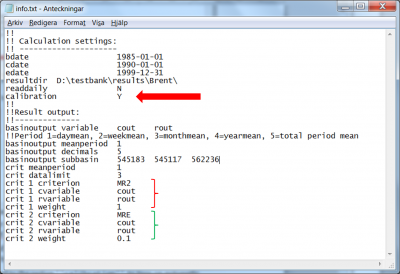
Ymust be passed to the model by the codecalibrationto turn on automatic calibration (red arrow in Fig 1). - An objective function must be specified by means of the performance criteria it is composed of. Such a composite criterion, are constructed by linear combination of the already implemented, performance criteria, like:
where are predefined performance criteria, and
are relative weighting factors. The available performance criteria and their id are listed here. The criterion id, the HYPE variable ID of the computed and recorded variables to compare, as well as the period over which the variables are averaged before calculating the criterion, is specified for each performance criterion to be included in the objective function (see the block of data marked in red and green in Fig 1). For details on format see the description of the info-file.
In the example of Fig 1 the Nash-Sutcliffe efficiency (MR2) and relative error (MRE) are calculated for daily discharge (cout and rout are compared on meanperiod 1). The two criteria are weighted together. Most weight is put on MR2 and a little on the volume error. A small weight on relative error is usually enough to minimize the volume error but still get a good NSE. In the example all observations found in Qobs.txt are used to calculate the objective function. If more than one station is found, the MR2 criterion will use the average of each station’s NSE.
Description of all available criteria and their equations can be found in the wiki (criteria equations). Several performance criteria are available in HYPE, because they are useful for different situations and variables. For example correlation (MCC) can be used if you want to calibrate on timing, but not bother with the average value, spatial criteria can be used if you want to focus on the spatial variation, and Nash-Sutcliffe efficiency adjusted for bias (MNW) can be used for calibrating water stage to avoid artefacts coming from different height systems.
Specification of calibration - optpar.txt
The file optpar.txt defines what kind of optimization to be done. There are several different optimization methods, each with their special settings and numerical parameters. The file also specifies which model parameters to calibrate, as well as numerical specifications for those. The file is divided in three sections:
- A header of no importance, occupying the first line; HYPE does not read this.
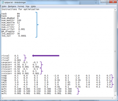
- 20 lines are available for the specifications of settings and numerical parameters required by the optimization methods; see blue block of data in Fig 2. The input specified in this part of the file is explained for each optimization method in section Specification of calibration parameters - optpar.txt and on the wiki-page describing optpar.txt. Note that these settings are case sensitive and that the numerical values start on position 12.
- The model parameters to be calibrated, the listing starting on the 22nd line of the file. HYPE expects the parameter listing to start at line 22 exactly, it is therefore of tremendous importance to do exactly so; see the purple arrow in Fig 2. HYPE expects three lines for each model parameter, each line starting with the parameter name (all parameters are listed on the wiki page for par.txt); see purple blocks of data in Fig 2. The parameter listing specified in this part of the file is explained in next section Specification of calibration parameters - optpar.txt.
Specification of calibration parameters - optpar.txt
Which model parameters to calibrate automatically is an important decision. Choosing many parameters may take long time to simulate. Some parameters may be unsuitable to calibrate with a certain method, e.g. threshold parameters are tricky for the Brent method which assumes parabolic behaviour close to a value.
For each parameter to calibrate HYPE expects a calibration interval. In addition some methods require determination accuracy or (for the DEMC method) a parameter specific factor to scale the random noise added to the proposed next-generation of this parameter. Therefore, independent on method, three lines of values are passed for each optimization parameter, all starting with the parameter name: the calibration interval lower boundary on the 1st line, the calibration interval upper boundary on the 2nd line, and the accuracy or factor on the 3rd line, all written in decimal form.
Example: general parameter
The first parameter, in the case presented in Fig 2, is a general model parameter called rivvel (see first purple block in Fig 2). A general parameter has one value for the whole model set-up. The rivvel parameter determines the celerity of flood in the watercourse. We would like to vary it between 0.5 m/s up to 2.0 m/s. Thus we set it to the interval [0.5, 2.0]. Further we would like to determine its optimal value with no larger accuracy than three decimals. The parameter rivvel appears on three consecutive lines, starting on the 22nd line (purple arrow in Fig 2); the parameter being a scalar, each line holds only one value:
- the lower calibration interval boundary, 0.5, on line 22
- the upper calibration interval boundary, 2.0, on line 23
- the required 3-decimal precision, 0.001 on line 24
Using for each model parameter the exact same format of three lines, the corresponding calibration information is passed to the optimization methods; see purple blocks in Fig 2.
Example: one-dimensional parameters
A type of parameter that is common in calibration is the correction parameters. These are often one-dimensional parameters depending on region, for example cevpcorr (second purple block in Fig 2). This parameter adjusts the evaporation parameter up or down as compared to the value(s) given in the par.txt file. If we want to vary the evaporation between 5% of its value up to 195% of its value, we set the interval to [-0.95, 0.95]. This way of calibrating the evaporation by a correction parameter allow:
- the evaporation to keep its, in par.txt defined, variation between land-uses while adjusting the overall evaporation, and
- adjust the evaporation differently for, in this case three, different regions.
The format for one-dimensional parameters is the same as described above; three lines with minimum, maximum, and precision/factor on consecutive lines. The dimension of parameters may be parameter regions (as for cevpcorr above), or e.g. land-use, soil type or other. In the case of one-dimensional parameters, we might want to calibrate only a few of the values, e.g. only the dominant land-uses, but not all of them. To avoid calibrating the parameter value associated with a certain land-use, it is sufficient to set the lower and upper interval boundaries to the same value. The calibration algorithm will then ignore this parameter value, since its variation interval has a zero length. In this case the value specified in par.txt will be used.
The land-use dependent parameter ttmp in Fig 2 illustrates how to calibrate a few of the values of a one-dimensional parameter. Suppose the 5th and 7th land-uses dominate heavily the model setup. Since other land-uses contribute only marginally to the model, modifications of their ttmp-values will have little impact on the simulations and it is therefore reasonable to calibrate only the 5th and 7th ttmp-values. Suppose further that we expect the parameter values for those two land-uses to take a value in the interval [-2, 2], and that we wish a parameter value determination down to one decimal.
To do so, we set the lower and upper interval boundaries to equal values (any values, as long as they are equal) for all values, except the 5th and 7th where we set -2 as lower boundary, and 2 as upper boundary; finally we write 0.01 of the 5th and 7th columns on the 3rd line, in order to enforce determination by optimization of the parameter values to one-decimal precision.
Specification of optimization method and settings - optpar.txt
We discuss here method by method the upper part of the file optpar.txt, marked in blue in Fig 2. A comprehensive listing of all settings is found on the wiki-page of optpar.txt. Note that the codes and values of the settings are all case sensitive, while the calibration parameters are not. Note also that the values of the settings start on position 12 of the lines.
Basic Monte-Carlo method (task MC)
The basic Monte-Carlo method will randomly sample parameters from a uniform distribution within the parameter space. The Monte-Carlo method requires the specification of two numerical parameters. These are the number of Monte-Carlo simulations to make and how many of them to save and print out results for. The best or the best few will then be kept track of during the execution.
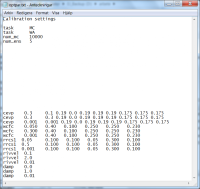
Suppose we want to perform a simple Monte-Carlo sampling of the criteria surface depending on the five model parameters cevp, wcfc, rrcs1 (for these three only the first value in the vector is calibrated), rivvel and damp. We require 10000 model runs and will keep the 5 best simulations.
- The task-flag for the basic Monte-Carlo method is
MC; see line 3 in Fig 3. - The task-flag
WAis optional. It forces HYPE to print out the performance results of all simulations in an output file called allsim.txt. The performance result of the best simulations will always be printed in the output file bestsims.txt. - The total amount of model runs is passed with the flag
num_mc. In the present example the command readsnum_mc 10000, see line 5 in Fig 3. - The amount of best runs to retain is passed with the flag
num_ens. In the present example the command readsnum_ens 5, see line 6 in Fig 3.
The specification of calibration parameters start on line 22. List the model parameters in no particular order, but with three rows for each parameter. The precisions specified in the parameter listing part are not used by the sampling method, but it is required for HYPE to interpret the optpar.txt file correctly.
Progressive Monte-Carlo method with parameter space limited by best found so far (task BP)
For this progressive Monte-Carlo method the Monto-Carlo simulations is done in stages with reduced parameter space in between the stages. The parameter space is reduced based on the best parameters found so far. For each stage, the parameter space is reduced to as small space as possible still containing all the best points, and this space is sampled for the next stage.
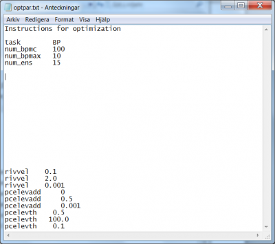
The method requires the specification of a few settings and numerical parameters. Suppose we want to perform a progressive Monte-Carlo sampling of the criteria surface depending on the three model parameters rivvel, pcelevadd and pcelevth. We require 100 model simulations per stage and 10 stages where the 15 best runs are retained to form the parameter space for the next stage (for a total numerical work of 100 x 10 = 1000 model runs).
- The task for this progressive Monte-Carlo method is set with the flag
BP(“bounded parameter space”); see line 3 in Fig 4. - The amount of model runs per stage is passed with the flag
num_bpmc. In the present example the command readsnum_bpmc 100, see line 4 in Fig 4. - The number of stages is passed with the flag
num_bpmax. In the present example the command readsnum_bpmax 10, see line 5 in Fig 4. - The number of best runs to retain to determine the parameter space for the next stage is passed with the flag
num_ens. In the present example the command readsnum_ens 15, see line 6 in Fig 4.
The specification of calibration parameters start on line 22. List the model parameters in no particular order, but with three rows for each parameter. The precisions specified in the parameter listing part are not used for the task, but required for HYPE to interpret the optpar.txt file correctly.
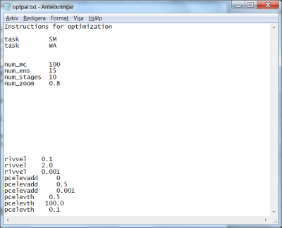
Progressive Monte-Carlo method with parameter space reduced in stages (task SM)
For this progressive Monte-Carlo method the Monto-Carlo simulations is done in stages with reduced parameter space in between the stages. The parameter space is reduced based on the best parameters found so far. For each stage, the parameter space is reduced by a percentage compared to the size of the previous stage. The reduced space is centred around each best point. The thus defined reduced parameter spaces are sampled in the next stage.
The progressive Monte-Carlo method requires the specification of a few settings and numerical parameters. Suppose we want to perform a progressive Monte-Carlo sampling for the three model parameters rivvel, pcelevadd and pcelevth. We require 100 model runs per stage and per center, 10 stages where the 15 best runs are retained as center for the next stage (for a total numerical work of 100 x 10 x 15 = 15000 model runs), and we want to shrink the parameter space radius by 20% at each stage.
- The task for the progressive Monte-Carlo method is set by the flag
SM(“staged Monte Carlo”); see line 3 in Fig 5. - The task with the flag
WAis optional. It forces HYPE to print out the performance results of all simulations in an output file called allsim.txt. The performance result of the best simulations will always be printed in the output file bestsims.txt. - The amount of model runs per center is passed with the flag
num_mc. In the present example the command readsnum_mc 100, see line 7 in Fig 5. - The amount of best runs to retain as center for the next stage is passed with the flag
num_ens. In the present example the command readsnum_ens 15, see line 8 in Fig 5. - The amount of stages is passed with the flag
num_stages. In the present example the command readsnum_stages 10, see line 9 in Fig 5. - The parameter space contraction factor is passed with the flag
num_zoom. In the present example, since we want to reduce the parameter spaces with 20% at each stage, 80% are retained and therefore the command readsnum_zoom 0.8, see line 10 in Fig 5.
The specification of calibration parameters start on line 22. List the model parameters in no particular order, but with three rows for each parameter. The precisions specified in the parameter listing part are not used by the method, but required for HYPE to interpret the optpar.txt file correctly.
2-parameters organized scan (task SC)
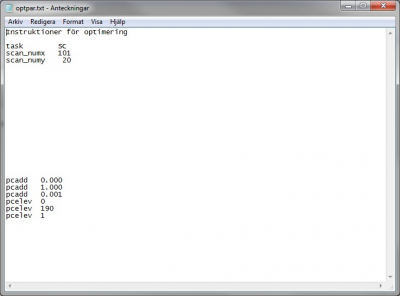
The 2-parameters organized scan does not require many settings; only 3 method-dependent flags and parameters have to be specified. We illustrate here the method to perform the regularly-spaced sampling of the criteria surface as dependent on the model parameters pcadd and pcelev. Assume that we require 101 sampling points of the model parameter pcadd, which is allowed to vary within the interval [0, 1], and 20 sampling points of the model parameter pcelev, which is given the bounds [0, 190]. The total numerical work thus includes 101 x 20 = 2020 model runs.
- The regularly-spaced sampling is triggered by the task-flag
SC; see line 3 in Fig 6. - The amount of parameter values to be taken for the first parameter has the flag
scan_numx. If the model parameterpcaddis coming first in the parameter listing, line 4 of the file readsscan_numx 101, see Fig 6. - The amount of parameter values to be taken for the second parameter has the flag
scan_numy. Therefore, in the example line 5 readsscan_numy 20.
The specification of calibration parameters start on line 22. Needless to say, the order of the model parameters in the parameter listing must be consistent with the order of the numerical parameters scan_numx and scan_numy: specify the bounds for pcadd first, then for pcelev. The precisions specified in the parameter listing part are not used for the sampling task, but required for HYPE to interpret the optpar.txt file correctly.
Differential Evolution Markov Chain method (task DE)
The Differential Evolution Markov Chain (DEMC) introduces uncertainty estimate in the Differential Evolution (DE) optimization algorithm by applying the Metropolis-Hastings acceptance criteria, and by adding a random number in the DE proposal generation. Another way of describing DEMC is that it is a simplified version of MCMC, where the DE proposal generation is used instead of the otherwise cumbersome MCMC jumps based on covariance and multivariate normal distributions. The genetic DE algorithm overcomes the difficult jump generation of MCMC by generating the proposal directly from the current populations. The advantage of DEMC versus plain DE is both the possibility to get a probability based uncertainty estimate and a better convergence towards the global optima. A description of DEMC can be found in ter Braak (2006) and in Rönkkönen et al. (2009).
The HYPE Differential Evolution Markov Chain (DEMC) optimization method has six numerical parameters that can be set.
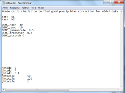
- The task for the DEMC method is set by the flag
DE; see line 3 in Fig 7. - The task for writing the simulation results for the best parameter sets is set by the flag
WS; see line 4 in Fig 7. This will write the basin-, time- or mapfiles asked for in info.txt for the best parameter sets (the number of best sets is set byDEMC_npop, se below) and the median parameter of these. - The number of generations can be specified; the total number of simulations will be the number of generations times the population size. The number of generations should be high enough to get convergence. The corresponding code is
DEMC_ngen. In the example of optpar.txt file shown in Fig 7, the 6th line indicates that the user wants 30 generations. - The size of the population can be specified by the code
DEMC_npop. The number has to be at least 3 for the method to work, and it should be at least 2*number of optimized parameters. In the example of optpar.txt file shown in Fig 7, the 7th line indicates that the user wants 10 members of the population. - The derivation of a new parameter set to be tested (the mutation) is governed by “gammascale”, which determine how much two randomly selected parameter sets will contribute to the new parameter set. The gammascale is set by the code
DEMC_gammascale. The new parameter set will keep most of the old parameter values if a low scaling value is chosen. The value sets the scaling of the default jump. Use 1 if you want quick convergence, risking too low acceptance frequency. Use « 1 if it’s a tricky problem. In the example of optpar.txt file shown in Fig 7, the 8th line indicates that the user wants 0.5 for scaling. - The derivation of a new parameter set to be tested (the mutation) is also governed by the code
DEMC_sigma. “Sigma” and the parameter precision determines how much a random perturbation will influence the new parameter set. “Sigma” is the base of the perturbation. The value is the standard deviation of the sample error. Set to 0 if you don’t want to use it. Default is 0.1. The sigma value is multiplied with 3rd-row value for each parameter (the precision) to determine the size of the random perturbation. - The probability to use the new parameter set is governed by the code
DEMC_crossover, which is the probability to not use the mutated parameter values. Use 1 to always test the mutation (default), or < 1 to cross over some parameter values from parent generation (recommended if you have large number of parameters). In the example of optpar.txt file shown in Fig 7, the 9th line indicates that the user wants 40% probability to keep the previous/parent parameter set and not to use the mutation. - As default, only new parameter sets with better optimization criterion is accepted for the next generation. The code
DEMC_accprobis used to switch on the possibility to accept also less good parameter sets. If used, a proposed parameter set is accepted with increasing probability the better its performance is compared to the best parameter set so far. Set to 0 to only accept proposals with better performance than the parent generation (default), set to 1 to turn on the probability to accept worse proposals. In the example of optpar.txt file shown in Fig 7, the 10th line indicates that the user wants new generations to be better.
The specification of calibration parameters start on line 22 in optpar.txt. Listing of the model parameters subject to optimization is achieved as described above. The model parameters are listed in no particular order, but with three rows for each parameter. The precisions specified in the parameter listing part are used by the DEMC method to scale the random perturbation of the generation of a new proposed parameter set.
Brent method (task BN)
The Brent method optimizes the parameters iteratively. One iteration is composed of several steps. First the method optimizes one parameter at the time. Each parameter is optimized with a line search algorithm. After all parameters have been optimized separately, an optional step may be taken that optimize the parameter set along the line from the best point before the parameters optimizations and the new best point, i.e. a “diagonal” step. This optimization is done with the line search routine. Then the Brent method starts another iteration of optimizing the parameters one after the other. This continues until one of several interruption criteria is fulfilled.
The Brent method requires the specification of a few settings; the different method interrupters, the flag for using of the diagonal step, and the numerical parameters for the line search routine. In addition a file with starting values of the parameters is required. For a given set of model parameters, optimization of the model setup by the Brent method is achieved by specification of the following:
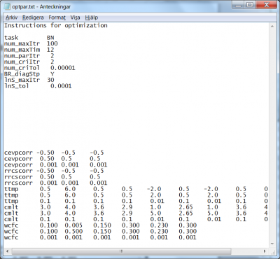
- The task for the Brent method is set by the flag
BN, for “Brent New”; see line 3 in Fig 8. - A maximum amount of iterations can be specified; if the optimization procedure reaches this amount, it automatically exits; the corresponding code is
num_maxItr. If the example of optpar.txt file shown in Fig 8, the 4th line indicates that the user wants the method to stop if it reaches 100 iterations. - Similarly, a maximum amount of computation hours for the method can be specified, by means of the code
num_maxTim. In the example given in Fig 8, the user wants the method to stop after 12 hours; see 5th line of the file. Default is 72 hours. - If no model parameter values change, according to the prescribed precision (3rd line in the model parameter listing for each parameter), for a certain amount of iterations the method exits. This amount of iteration is passed to the method by means of the code
num_parItr. In the example of Fig 8, the user requires the method to stop if no model parameter values change by more than the specified precision for the last two consecutive iterations. - Similarly, if the simulation optimization criterion does not change more than a given precision during a given amount of consecutive iterations, the method will exit. The amount of iterations is passed by means of the code
num_criItr, while the criteria precision is passed by the codenum_criTol. In the example of Fig 8, the user requires method exit if the criteria as not changed by more than 0.00001 over the last two consecutive iterations. - The diagonal step at the end of each iteration over all parameters is enforced by the setting the flag for
BR_diagStp. The code takes the valuesYfor yes, orNfor no; see the 9th line of the file in Fig 8. - For each parameter optimization a line search operation is performed, and a maximum amount of iterations for the line search can be specified by the code
lnS_maxItr. In the example at hand, maximum 30 line search iterations are allowed; see the 10th line of the file in Fig 8. - Similarly, for each line search operation, a relative tolerance for search interval contraction can be specified by means of the code
lnS_tol. In the example of Fig. 8, the line search interval is not allowed to be shorter than 0.0001.
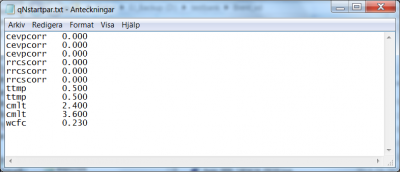
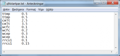
The specification of calibration parameters start on line 22 of the optpar.txt file. Listing of the model parameters subject to optimization is achieved as described above. The order in which the model parameters are listed in optpar.txt may be relevant for the result, since they will be optimised one by one in this order. In addition they must be listed in the same order in the qNstartpar.txt file. This file gives the starting parameter values for the line search in the Brent routine.
Quasi-Newton methods (task Q1 and Q2)
The quasi-Newton methods optimise all parameters at the same time. The direction of the search is determined by the gradient of the criteria surface at the point of the current best parameters. The parameter set is optimized with the line search routine along the line determined by the gradient. The gradient can be estimated in three different ways in HYPE, the two quasi-Newton methods described in this section and the one called steepest descent in the next section. The optimization continues until one of several interruption criteria is fulfilled.
Calculating the gradient for the quasi-Newton method involves updating the inverse Hessian matrix. This can be done by two methods, both described in Nocedal and Wright (2006). Task Q1 uses the DFP (Davidon-Fletcher-Powell) method and task Q2 uses the BFGS (Broyden-Fletcher-Goldfarb-Shanno) method.
The quasi-Newton methods require the specification of a few settings; different method interrupters, numerical parameters for the calculation of the numerical derivative, and numerical parameters for the line search routine. In addition a file with starting values of the parameter set is required. For a given set of model parameters, optimization of the model setup by a quasi-Newton method is achieved by specifying the following:
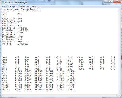
- The task for the quasi-Newton methods are the flags
Q1orQ2. Choose one of them. In the example method Q2 is used, see line 3 in Fig 10. - A maximum amount of iterations can be specified; if the optimization procedure reaches this amount, it automatically exits. The code to set the maximum iterations is
num_maxItr. For the example of optpar.txt file shown in Fig 10, the 4th line indicates that the user wants the method to stop if it reaches 500 iterations. - Similarly, a maximum amount of computation hours for the method can be specified, by means of the code
num_maxTim. In the example given in Fig 10, the user wants the method to stop after 240 hours; see 5th line of the file. - If no model parameter values change, according to the prescribed precision (3rd line in the model parameter listing for each parameter), for a certain amount of iterations the method exits. This number of iteration is passed to the method by means of the code
num_parItr. In the example of Fig 10, the user requires the method to stop if no model parameter values change by more than the specified precision for the last 8 consecutive iterations. - Similarly, if the optimization criterion does not change more than a given precision during a given amount of consecutive iterations, the method will exit. The amount of iterations is passed by the code
num_criItr, while the criteria precision is passed by the codenum_criTol. In the example of Fig 10, the user requires method exit if the criteria as not changed by more than 0.00001 over the last 15 consecutive iterations. - A tolerance for the gradient to be considered zero, i.e. an optimum reached, can be specified by the code
QN_nrmTol. In the example, the user defines it to 0.000001; see 9th line of the file in Fig 10. - When the gradient is to be estimated for a parameter set, simulations for a few points close to the current parameter set are made and used to calculate the numerical derivative. These points are offset from the midpoint parameter values based on each parameter's calibration interval, and a factor (default is 0.02, i.e. 2% offset). The offset for calculation of numerical derivative can be specified by the code
QN_pctDerv. In the example, the user defines it to 0.015; see 10th line of the file in Fig 10. - The number of points used to calculate the numerical derivative is called the numerical derivative stencil type (2, 4, 6 and 8 are allowed). The stencil type determines the order of accuracy of the numerical derivative, e.g. 2-stencil is 1st order accurate, 4-stencil is 2nd order accurate, etc. The stencil type can be specified by the code
QN_stencil. In the example, the user defines it to 2; see 11th line of the file in Fig 10. - The line search in the optimal direction may be limited within the given parameter intervals by a factor multiplied by the interval. Lambda is the name of the current direction and step length to be searched (according to the QN algorithm). If the step length and factor are both one, the whole suggested parameter interval is searched, and the offset points used to calculate the numerical derivative may end up outside the chosen parameter calibration interval. Therefore a factor less than one may be set. The factor can be specified by the code
QN_lambMax. In the example, the user defines it to 0.95; see 12th line of the file in Fig 10. - The actual maximum step length that the line search are allowed to take in the optimal direction, i.e. maximum value of lambda, is determined by the parameter limits, the direction vector and its length (i.e. the maximum step length according to the QN algorithm), and an in optpar.txt set factor for increasing the step length. The factor for increasing the step length can be specified by the code
QN_lambAcc. The default value of the factor is 1.618, consistent with golden ratio line search algorithm. The iteration process may thus be accelerated. In the example, the user defines it to 4.0; see 13th line of the file in Fig 10. - For each line search operation, a maximum amount of iterations can be specified by the code
lnS_maxItr. In the example at hand, maximum 100 line searches are allowed; see the 14th line of the file in Fig 10. - For each line search operation, a relative tolerance for search interval contraction can be specified by means of the code
lnS_tol. In the example of Fig 10, the line search interval is never allowed to be shorter than 0.000001.
The specification of calibration parameters start on line 22 of the optpar.txt file. Listing of the model parameters subject to optimization is achieved as described above. The order in which the model parameters are listed in optpar.txt is relevant for the qNstartpar.txt file; they must be listed in the same order. This file gives the starting parameter values for the line search in the quasi-Newton method.
Steepest descent method (task SD)
The steepest decent method is a special case of the quasi-Newton methods. Like the other quasi-Newton methods, it iteratively optimises all parameters together. The parameter set is optimized with the line search routine and the direction of the search is determined by the gradient of the criteria surface. The optimization continues until one of several interruption criteria is fulfilled.
Calculating the gradient for the quasi-Newton method involves updating the inverse Hessian matrix. This step is skipped for the steepest descent method, because it approximates the inverse Hessian matrix as a unit matrix.
The steepest descent method requires the specification of a few settings; the different method interrupters, numerical parameters for the calculation of the numerical derivative, and the numerical parameters for the line search routine. In addition a file with starting values of the parameter set is required. For a given set of model parameters, optimization of the model setup by this method is achieved by specification of the following:
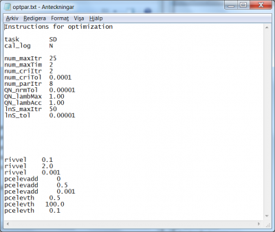
- The task for the steepest descent methods is set by the flag
SD, see line 3 in Fig 12. - The calibration.log file is written automatically, but the writing can be turned off with a flag
cal_logset toN, see line 4 in Fig 12. - A maximum amount of iterations can be specified; if the optimization procedure reaches this amount, it automatically exits. The code to set the maximum iterations is
num_maxItr. In the example of optpar.txt file shown in Fig 12, the 6th line indicates that the user wants the method to stop if it reaches 25 iterations. - Similarly, a maximum amount of computation hours for the method can be specified by the code
num_maxTim. In the example given in Fig 12, the user wants the method to stop after 2 hours; see 7th line of the file. - If the objektive function does not change more than a given precision during a given amount of consecutive iterations, the method will exit. The amount of iterations is passed by the code
num_criItr, while the criterion precision is passed by the codenum_criTol. In the example of Fig 12, the user requires method exit if the criterion as not changed by more than 0.0001 over the last 2 consecutive iterations. - If no model parameter values change, according to the prescribed precision (3rd line in the model parameter listing for each parameter), for a certain amount of iterations the method exits. This number of iteration is passed to the method by means of the code
num_parItr. In the example of Fig 12 line 10, the user requires the method to stop if no model parameter values change by more than the specified precision for the last 8 consecutive iterations. - A tolerance for the gradient to be considered zero, i.e. an optimum reached, can be specified by the code
QN_nrmTol. In the example, the user defines it to 0.00001; see 11th line of the file in Fig 12. - When the gradient is estimated for a parameter set, simulations for a few points close to the parameter set are made and used to calculate the numerical derivative. These points are offset from the midpoint parameter values based on each parameter calibration interval, and a factor (default is 0.02, i.e. 2% offset). The offset for calculation of numerical derivative can be specified by the code
QN_pctDerv. In the example, the default is used. - The number of points used to calculate the numerical derivative is called the numerical derivative stencil type (2, 4, 6 and 8 are allowed). The stencil type determines the order of accuracy of the numerical derivative, e.g. 2-stencil is 1st order accurate, 4-stencil is 2nd order accurate, etc. The stencil type can be specified by the code
QN_stencil. In the example the default value 2 is used. - The line search in the optimal direction may be limited within the given parameter intervals by a factor multiplied by the interval. Lambda is the name of the current direction and step length to be searched (according to the QN algorithm). If the step length and factor are both one, the whole suggested parameter interval is searched, and the offset points used to calculate the numerical derivative may end up outside the chosen parameter calibration interval. Therefore a factor less than one may be set. The factor can be specified by the code
QN_lambMax. In the example, the user increases it to 1 (from the default value 0.9) to use the suggested interval; see 12th line of the file in Fig 12. - The actual maximum step length that the line search are allowed to take in the optimal direction, i.e. maximum value of lambda, is determined by the parameter limits, the direction vector and its length (i.e. the maximum step length according to the QN algorithm), and an in optpar.txt set factor for increasing the step length. The default value of the factor is 1.618, consistent with golden ratio line search algorithm. The iteration process may thus be accelerated. The factor for increasing the step length can be specified by the code
QN_lambAcc. In the example, the user defines it to 1.0; see 13th line of the file in Fig 12. - For each line search operation, a maximum amount of iterations can be specified by the code
lnS_maxItr. In the example at hand, maximum 50 line searches are allowed; see the 14th line of the file in Fig 12. - For each line search operation, a relative tolerance for search interval contraction can be specified by means of the code
lnS_tol. In the example of Fig. 12, the line search interval is never allowed to be shorter than 0.00001.
The specification of calibration parameters start on line 22 of the optpar.txt file. Listing of the model parameters subject to optimization is achieved as described above. The order in which the model parameters are listed in optpar.txt is relevant for the qNstartpar.txt file; they must be listed in the same order. This file gives the starting parameter values for the line search of the steepest descent method.
References
ter Braak, Cajo J. F. (2006). A Markov Chain Monte Carlo version of the genetic algorithm Differential Evolution: easy Bayesian computing for real parameter spaces. Stat Comput, 16:239-249, DOI 10.1007/s11222-006-8769-1
Nocedal J., and S.J. Wright (2006). Numerical optimization (second edition), Springer series in operational research, Springer 2006, Chapter 6.1 (p. 135-143)
Rönkkönen J., Li, X., and V. Kyrki (2009). The role of local and global search in solving problems with multiple global optima. Technical Report 110, Department of Information Technology, Lappeenranta University of Technology. ISBN 978-952-214-730-1
