Navigation
HYPE Documentation
Quick links to often-used pages:
HYPE links
HYPE OSC (model code)
HYPE Open data access
SMHI Hydrology Research Dep., main developer and maintainer of the HYPE model
Quick links to often-used pages:
HYPE OSC (model code)
HYPE Open data access
SMHI Hydrology Research Dep., main developer and maintainer of the HYPE model
This tutorial provides introductory guidelines for creating a HYPE model set-up in a new model domain. These guidelines cover the creation and formatting of mandatory and optional input files for a basic HYPE rainfall-runoff and nutrient turnover model. HYPE requires all input data as a set of formatted text files (e.g. model domain information, observation data, or calibration parameters). All input files mentioned in this tutorial are documented in detail in the file reference section of the HYPE documentation pages.
This tutorial is a minor part of the main tutorial for HYPE: Setting-Up HYPE
HYPE domains are spatially divided into sub-basins for which hydrological response units (HRUs) are derived. In order to create a HYPE model set-up, modellers will have to create a suitable sub-basin delineation based on a topographical database. SMHI provides the freeware GIS tool WHIST (World Hydrological Input Setup Tool) which is especially suited for setting up large HYPE domains. WHIST provides additional functionality, e.g. to calculate HRU fractions for each sub-basin, and a convenient file export in HYPE-conform formatting but users can choose any GIS software suitable to derive sub-basins and flow routing connections and build their HYPE set-up workflow around them.
The following links list further in-depth reading, complementary to this tutorial:
HYPE software is available from the following sites:
If sub-basins do not exist for the targeted model domain, or if the routing is not defined between them, this information has to be created for a HYPE model set-up.
SMHI has, as already mentioned, developed a software for this purpose called WHIST. Besides the software the WHIST pages include descriptions on how to create subbasins from hydrologically corrected topography data, import already existing subbasins, extract spatial information for each subbasin needed as input for the HYPE model and export of shapefiles of the created subbasin polygons and a GeoData file in HYPE format. A basic model and some exercises are also provided to get started and used to the WHIST interface.
The following sections outline the main steps which need to be taken to create a HYPE set-up in a new model domain.
HYPE model domains are divided into spatially delineated sub-basins. A hydrologically corrected gridded topographic database is used to derive the model domain (i.e. all sub-basin areas). The procedure is preferably controlled by the geographic location of gauging stations (so called “forced points”) and their documented catchment area. Before use, especially when using larger global databases, all data used should be quality checked and gauging stations used as forced points during delineation need to be adjusted to the river network of the used topography data. The delineation can then be forced to capture the gauging station at the subbasin outlet and then the possibility to calibrate the model against the observations is optimized, see Fig. 1 to Fig. 3. How big the adjustments are is dependent on the resolution of the elevation data and the quality of the gauging station metadata.
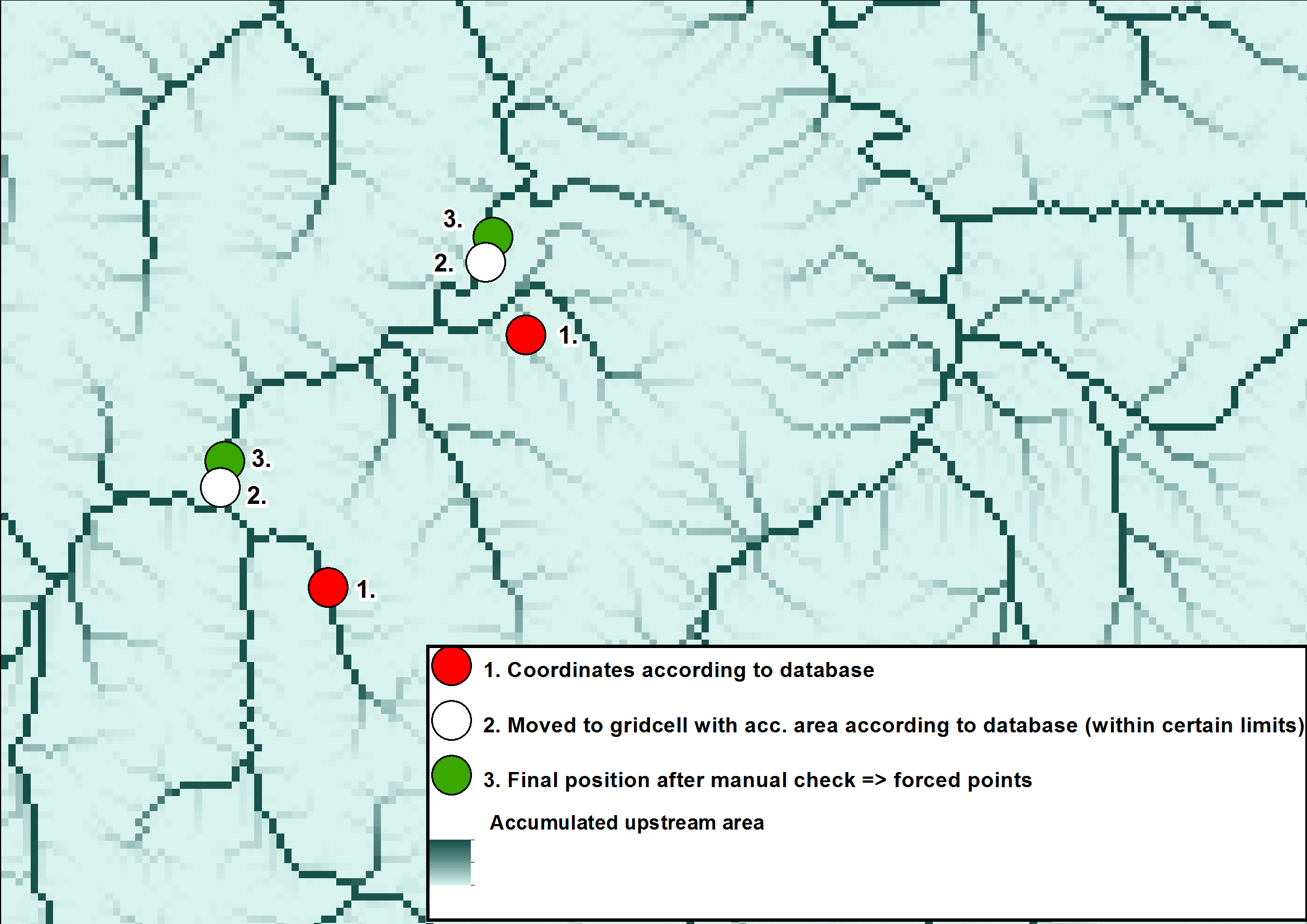 |
| Figure 1: Adjustment of gauging stations according to published drainage area. The flow accumulation data from Hydrosheds shows here the river network. |
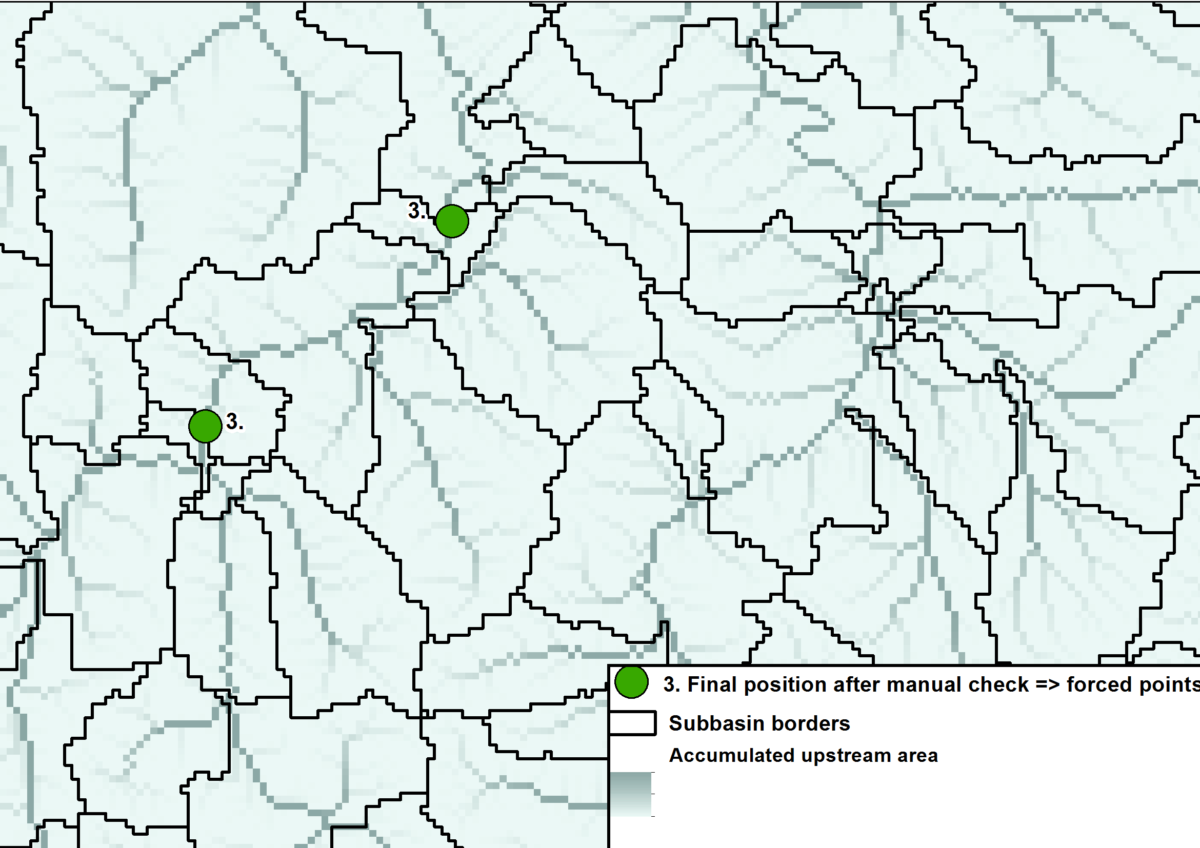 |
| Figure 2: The subbasins have been calculated and drawn. |
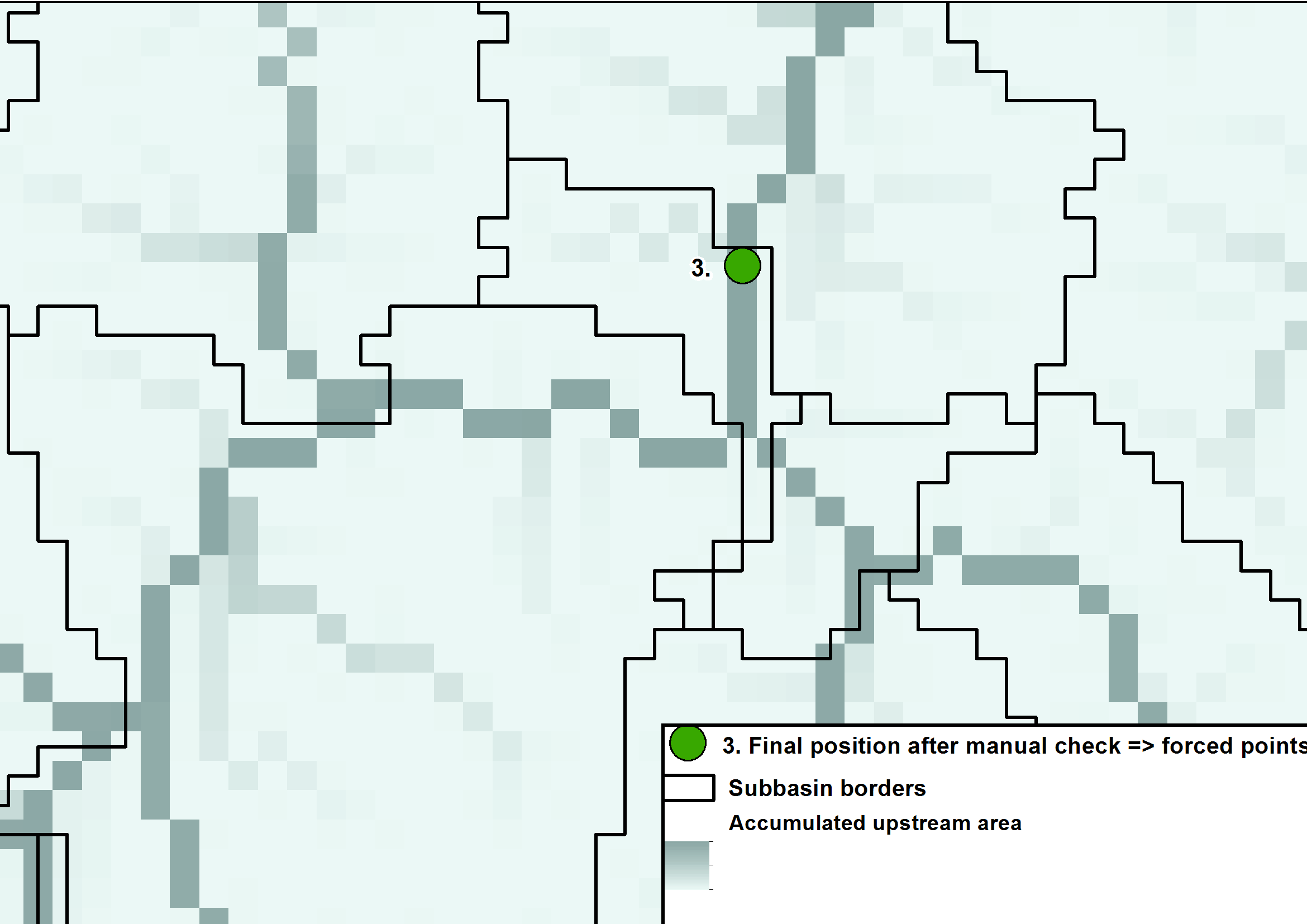 |
| Figure 3: The subbasin border is drawn to fit the outlet to the gauging station. |
Each subbasin must receive a unique subbasin ID (SUBID) and the SUBID of the subbasin next downstream (called MAINDOWN in HYPE) to explain the routing, see figure 4. This is mandatory for the model and described in GeoData.txt (more info here).
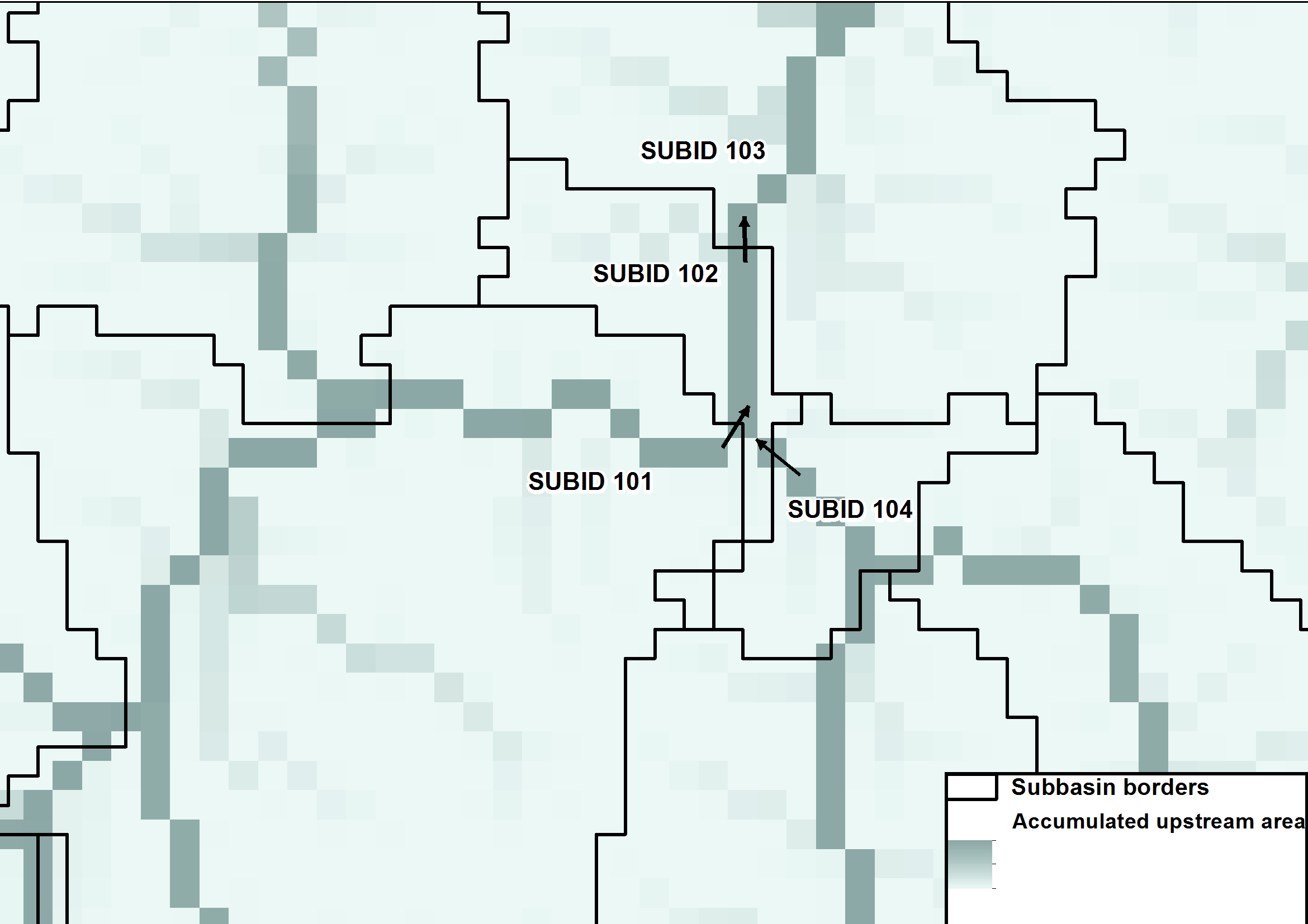 |
| Figure 4: Routing between sub-basins. SUBID 103 is next downstream to SUBID 102. SUBID 102 is next downstream to SUBID 101 and 104. |
Lakes can be included to the model in two ways: as local lakes (ilakes) or as outlet lakes (olakes) located at the main stream and at the outlet of a subbasin, see figure 5. The outlet lakes can be provided with individual rating curves and/or regulation schemes in LakeData.txt (more info here).
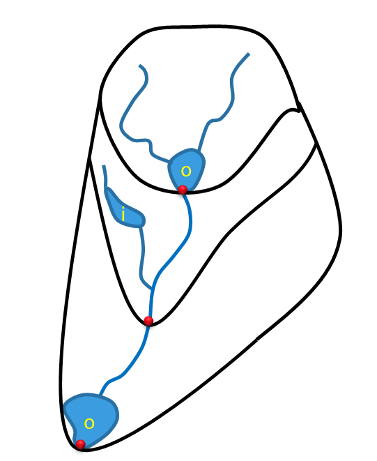 |
| Figure 5: Description of outlet lakes (o) and local lakes (i). |
The outlet lake can be modelled as a part of a subbasin (located at the subbasin outlet), as an individual subbasin (100 % lake) or as a so called Multibasin lake which covers several subbasins (but still with its outlet corresponding to the most downstream subbasin outlet), see figure 6. Multibasin lakes must be described in LakeData.txt to be correct represented. The two other types can either just have general parameters in the par.txt file or individual parameters in the LakeData.txt.
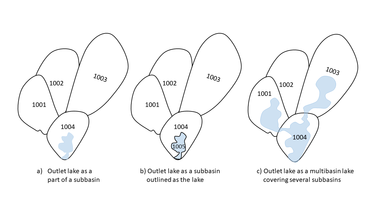 |
| Figure 6: Sub-basins should be drawn with their outlets fitting to the olakes outlet. The olake could either be totally within a larger subbasin (no need of exact shape of olake) drawn as its own subbasin (lake polygon needed) or cover several subbasins (multibasin olake). For all types of olakes the outlet of the lake should coincide with the subbasin outlet. |
Regardless of which outlet lake representation to choose it is necessary to use the (o-)lake outlet points as forced points when generating the subbasins.
Hydrological response units (HRUs) are derived for each subbasin. In HYPE the soil and landcover properties are combined into so called SLC's, Soil and Landcover Classes (for example forest + medium soils, open land + fine soils etc), see figure 7. The distribution of SLC classes for each subbasin is described in GeoData.txt and the SLC classes are defined in GeoClass.txt (more info here).
Keep landuse and soil classes essential and typical for the model domain but merge classes into a number you will manage to calibrate.
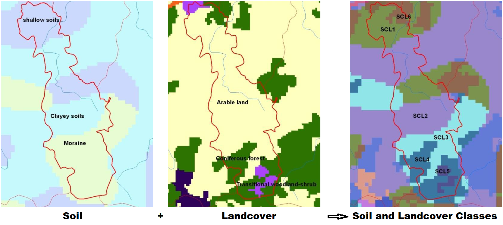 |
| Figure 7: Soil and landuse information is combined into SLC classes. Each subbasin is described with the proportion of the different classes in GeoData.txt. |
The model is forced by temperature (Tobs.txt) and precipitation (Pobs.txt) time series (mandatory) as a minimum. Temperature and precipitation can be corrected by elevation. The mean elevation of each sub-basin is included to the GeoData.txt file.
The separation of precipitation into rainfall and snow is usually done using air temperature threshold parameters, see Processes above ground in model description. However, it is also possible to force the model with a prescribed time series of snowfall fractions fraction in precipitation using the input-file SFobs.txt.
The default snowmelt model uses only air temperature as input. As an alternative, a snowmelt model based on temperature and radiationcan be used. In that case, shortwave radiation is either read from an input file SWobs.txt or estimated.
Read more about these processes in the model description.
The model could use different types of PET (potential evaporation) models (Alternative potential evaporation models). The different options for calculation of potential evapotranspiration requires additional forcing data, e.g. potential evaporation, extra-terrestrial radiation, daily min and max air temperatures, shortwave radiation, relative humidity, wind speed.
The HYPE code is continuously under development and new opportunities to force the model may be developed in the future. See http://hype.sourceforge.net/ for news.
There is an option to run water quality with HYPE. For modelling water quality, i.e. nitrogen and phosphorus leaching and transport, an additional file CropData.txt is required. CropData.txt consists of information on vegetation properties, e.g. average nutrient uptake, and crop management properties (e.g. fertilization amounts, sowing and harvesting days). Each line in CropData.txt holds information on a specific crop (or other vegetation) in a specific region (defined for each SUBID in GeoData.txt). Links between SLC and crops (main and secondary) are made in GeoClass.txt.
In addition, a few extra columns may be required in GeoData.txt. These include:
PointSourceData.txt holds information on point sources of nitrogen and phosphorus and in which SUBID they are discharged. Abstractions, e.g for municipality water supply, may also be handled in PointSourceData.txt.
These files are only necessary if nutrients are to be modelled.
All input files to HYPE are listed and described in detail in the HYPE file reference section of the online documentation.
Some of the setup and input data files described in this section of the tutorial are mandatory for every HYPE model setup: Mandatory input data
Always be careful to follow the described file formats.
GeoClass.txt is a file that defines the properties of the Soil and Landuse Classes (SLC) in geodata. Each class also need information about stream drainage depth, number of soil layers and soillayer thickness. Special classes as outlet lakes, local lakes, glaciers are defined and if nutrient will be simulated also crop type is necessary to define.
Figure 8 shows a typical GeoClass.txt file. The first three rows contain comments, here some class ID references for different columns. These rows are denoted with an exclamation mark “!”. The column heads on row 4 are also just comments and not necessary for HYPE since the order of columns is predefined.
The first column describes the SLC id. This id links geoclass to the SLC information in GeoData.txt. The second and third column describes the combination of landuse and soil in the SLC. Lakes (here: SLC 1 and 2) have 2 rows here. One for the special class 1 (outlet lake) and one for the special class 2 (internal lake). Glaciers also have a figure (3) in the special class column.
All classes have got a figure for the vegetation type. This is only used for the NP simulations though. Crops have got a tile-depth in this example. It describe the distance from soil surface to the tile drainage system. Drain depth is the distance from soil surface to local stream depth.
The last 4 columns describe the number of soil layers and the depth of these layers from soil surface to bottom of each soil layer.
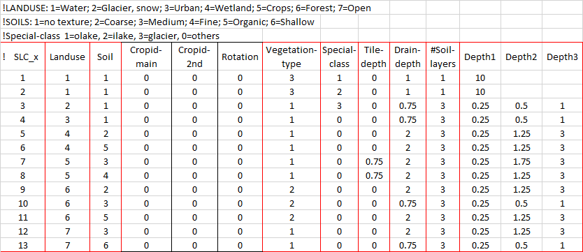 |
| Figure 8: Typical GeoClass.txt structure. |
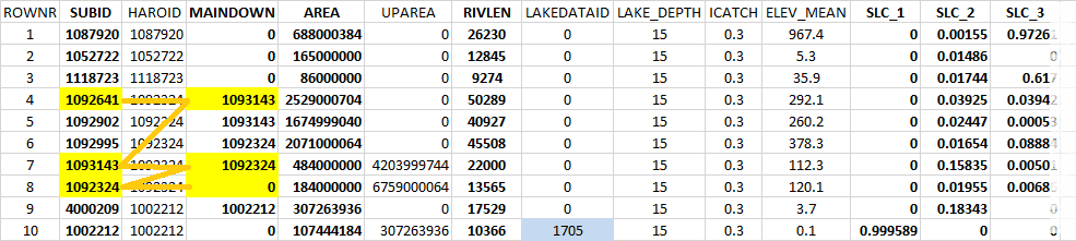
Geodata.txt holds information about the subbasins. One subbasin on each row. Necessary information is an identification number (subid), subbasin area (area), and area fractions of different classes (slc_nn). Other information that is often included in GeoData.txt is the routing, i.e. subid of downstream subbasin (maindown), main river length (rivlen), mean elevation (elev_mean) and outlet lake average depth (lake_depth). For nutrient simulations also crop region (region), atmospheric deposition (e.g. precipitation concentration of inorganic nitrogen, wetdep_n) and diffuse sources from rural households are common. See GeoData.txt for a comprehensive reference on GeoData.txt columns.
The structure of a GeoData.txt files is shown in Fig. 9. The first column holds the ROWNR to keep the order of the rows since the subbasins have to be ordered in a downstream sequence starting at headwaters and ending at outlet basins. The columns SUBID and MAINDOWN (0=outlet to the sea) hold the routing information (see the yellow marked cells for an example of how the routing is given).
The columns may be in any order and the sum of the SLCs for each subbasin should be =1. If your model contain a LakeData.txt file for tailored data on lake properties, you need to link to this file in the column named LAKEDATAID (see blue cell). HAROID (main river basin ID) is not mandatory but if your model cover many river basins it is handsome to see which subbasins belong to which main river basin. UPAREA (the total upstream area of the subbasin) is not mandatory either, but also useful to easily see if it is a large or small area contributing to the actual subbasin. HAROID and UPAREA are exported from WHIST by default. See the GeoData.txt for more information about the GeoData columns.
 |
| Figure 9: An example of GeoData.txt file structure. |
It is necessary that the subbasins are ordered in a downstream sequence. HYPEtools includes a function SortGeoData() for this purpose.
When GeoData.txt has been constructed it is always a good idea to check the tailoring of the data. Join the GeoData.txt to the subbasin shapefile and produce some maps for spatial check, i.e. ELEV_MEAN, summerized LandUse and Soilclasses. A function GroupSLCClasses() from HYPEtools can be helpful. To check the routing you can map each sub-basin's catchment area (from WHIST: AREA+UPAREA, from HYPEtools: SumUpstreamArea()) and get a view of the network.
Precipitation (mm/time step) and temperature time series (°C/time step) are needed to force the model. Pobs.txt and Tobs.txt files are therefore mandatory. If you use complementary data needed for other PET/snowfall/snowmelt models other than standard, these options can be chosen in info.txt, see model options.
Choose source database. Take into account accuracy, resolution, and also final use of model, i.e. operational forecasting, climate modelling, local studies, etc. These all should affect the choice.
Create links from SUBID in HYPE to grid square in input data set using WHIST or another GIS software or method. Depending on grid and sub-basin sizes, area-weighted averaging of gridded forcing data might be prudent.
Create Pobs.txt and Tobs.txt files. The forcing data can either have each SUBID as column header or an independent PobsID/TobsID, e.g. the original forcing data ID. If PobsID and TobsID are used, the link between these and the SUBIDs is described in ForcKey.txt.
The structure of forcing data files is illustrated in Fig. 10 and Fig. 11.
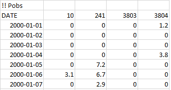 |
| Figure 10: Part of Pobs.txt. First column is used for dates, following columns for observed data. Column headers are either SUBID (if you have a unique observation for each SUBID) or POBSID (if you use ForcKey.txt and several SUBIDs use the same time series). |
 |
| Figure 11: Part of Tobs.txt. First column is used for dates, following columns for observed data. Column headers are either SUBID (if you have a unique observation for each SUBID) or TOBSID (if you use ForcKey.txt and several SUBIDs use the same time series). |
Make sure there is an elevation correction in par.txt for temperature and precipitation if necessary (will depend on your input data sets, resolution, geography etc).
Suggestions for quality assurance of forcing data:
ForcKey.txt is a key file for linking forcing data ID to SUBID. This file is not necessary if SUBIDs are used in Pobs.txt and Tobs.txt. If ForcKey.txt is used, this has to be stated in the info.txt with readobsid = y. If several subbasins are linked to the same Pobs and Tobs time series (e.g. if the resolution of the forcing data is coarser than the average size of the subbasins) the use of a ForcKey file can decrease the size of the Pobs and Tobs files and then also the running time of the model.
The structure of a typical ForcKey.txt file can be seen in Fig. 12.
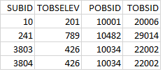 |
| Figure 12: Example of ForcKey.txt. The first column describes the SUBID. The next column the elevation for air temperature observation in meter. The third and fourth columns show the TOBSID and POBSID used in Pobs.txt and Tobs.txt. Here the last two subbasins are linked to the same POBSID and TOBSID. |
This file contains all model settings for a model run and this provides the main user interface. Here, the modeller can define e.g. simulation start and end dates along with spin-up periods, which output files to print and which performance statistics to calculate. Users can also choose different options for model components, e.g. for evaporation and snowmelt modules. All settings are entered as code-value pairs in info.txt.
There are many options, the HYPE file reference entry for info.txt provides a comprehensve description of options and syntax. In figure 13 you can find a basic example of an info.txt file. The rows can be in any order and comment rows can be added using a double exclamation mark identifier '!!'.
For different type of output files see the file reference entries for output files. For different types of output variables see the file reference entries for output variables.
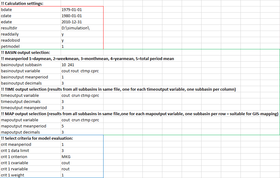 |
| Figure 13 (click to enlarge): info.txt example structure. Marked in red are codes to set model options, which are typically followed by codes describing output options (marked in green), and codes describing performance criteria options. |
The parameter file, par.txt, hold model parameters some of which can be calibrated. Some parameters are general, some landuse dependent, some soil dependent. There are also some parameters that can be tailored to certain given regions. See further information in the file reference entry for par.txt. There are also some suggestions on start values in the Quick Guide tutorial.
A simple example of the structure of the par.txt is described in Fig. 14. Parameters are soil-, landuse- or region-dependent. There are also general parameters used for the total model domain. Parameters dependent on soil and landuse classes have to be ordered in the same way as in the GeoClass.txt file. As you can see the par.txt file example in Fig 14 has the same number of landuse and soil parameters as described in the GeoClass file in Fig. 8. Region-dependent parameters are parameters which collectively alter groups of parameters and allow for regional tuning (super-parameters). Parameter regions for these have to be defined in GeoData.txt in a column named PARREG.
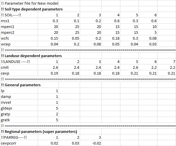 |
| Figure 14: A basic example of par.txt (click to enlarge). One row per parameter. Comment rows can be inserted using '!!'. |
There are many optional components in HYPE. Below we describe some of the most commonly used optional model components, lakes and reservoirs and bifurcations, which often have large impact on the hydrology in large-scale river basins. Others can be found among the tutorials (e.g. floodplains).
LakeData.txt is used to tailor rating curves and/or general regulation routines to the olakes. For use of LakeData.txt you need more specific information about lake depths, regulation volumes etc. For larger lakes and reservoirs around the world these can for example be found in the GLWD (Global Lake and Wetland Database) and GranD (Global Reservoir and Dam database) databases.
lakadataid is used in both GeoData.txt and LakeData.txt for this purpose.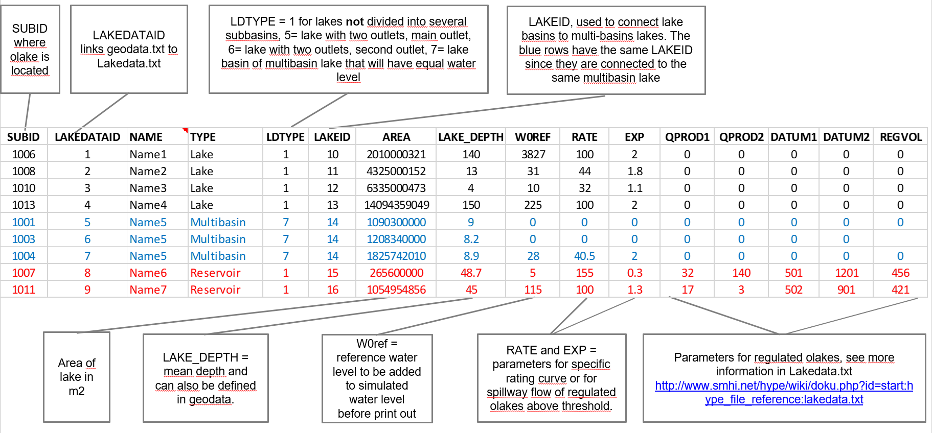 |
| Figure 15 (click to enlarge): Example of LakeData.txt. The LakeDataID is the link between GeoData.txt and LakeData.txt files. If a SUBID has a LakeDataID in GeoData.txt, the olake in this SUBID will be calculated according to the information in LakeData.txt. Black rows show some typical lakes, blue rows shows an example how to set up a multi-basin lake. The last blue row (also the outlet of the olake), keeps the rating and regulation parameters for the entire lake. The red rows show some typical reservoirs. See more information about this file in LakeData.txt. |
With this file it is possible to describe bifurcations and other water diversions in downstream direction. Read more about this file at BranchData.txt. Fig. 16 provides an example of a BranchData.txt file.
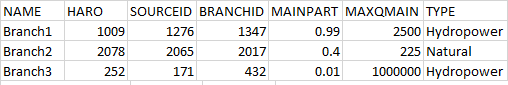 |
| Figure 16: BranchData.txt example. Sourceid is the SUBID with the bifurcation. Branchid is the SUBID of the receiving flow and this must be located in a row below the subbasin with bifurcation in GeoData.txt. Mainpart is the fraction of flow which flows in the main branch (not to branchid). Maxqmain is maximumflow in the main path. It is also possible to set limits for the branch path. The columns NAME and TYPE are just informative columns and can be excluded. |
For calibration and validation of the model, observed time series of discharge data are compiled in a file Qobs.txt. Other types of observations, e.g. nutrient concentrations or lake water levels are compiled in a file Xobs.txt.
Qobs.txt contains observations of discharge in m3/s for each time step. An example of Qobs.txt is given in Fig. 17.
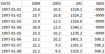 |
| Figure 17: Example of Qobs.txt . First column is used for the date of observation and must be continuous. Then each column have the SUBID the data is given for as header. Missing values should be given as -9999 since 0 will be interpreted as no flow. |
Suggestions for quality assurance in discharge observations:
The Xobs.txt file can contain observations of several selected variables, see more information in the file reference entry for Xobs.txt. An example of an Xobs.txt file is shown in Fig. 18.
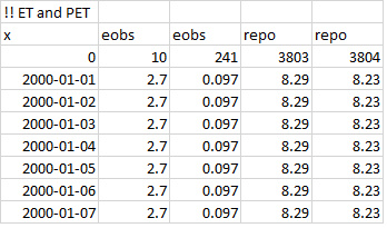 |
| Figure 18: An example of an Xobs.txt file with observed evapotranspiration and potential evaporation in mm/timestep. |
A HYPE model run is started by placing the HYPE executable file in the model folder and run it. Please read the information in the Quick Guide for details.
In Fig. 19 you can see an example of a HYPE model set up, just a collection of text-files and the executalbe HYPE code.
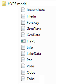 |
| Figure 19: Example of HYPE model set up. |
It is possible to save model states for model initialisation, e.g. to save computation time on spin-up periods or to provide comparable starting states in scenario analyses. Read more about this in the file reference entry for State_Save files.
HYPE provides three standard output file types for simulated data, one centered around single sub-basins, and two more centered around single output variables. There are further output files for water balances and model evaluation results. These are documented in detail in the Output Files section of the HYPE file reference.
Read more about the calibration options in the HYPE file reference section for calibration files.
